Learning Material
Introduction
Machine learning (ML) is growing in popularity not only within the realm of data science & statistics, but also throughout economics, healthcare, agriculture and more. ML techniques work to make predictions about future data, based upon models developed from sample (or training) data. As a whole ML techniques, can be divided into two main schools, supervised learning & unsupervised learning. With the main difference being the level of previous information provided. For supervised learning, this entails the tagging of data, typically identifying each variable as an input or output in relationship to another variable. Whereas, for unsupervised learning, this data is untagged, resulting in exploratory data analysis.
For the purpose of this session, we will focus on one form of supervised learning, that is tree-based models, and in particular decision trees. With tree-based models being suitable for many simple regression and classification problems, whilst being highly interpretable in their early stages.
Additionally, this session will use techniques and content discussed in An Introduction to Statistical Learning, with Applications in R by James, Witten, Hastie & Tibshirani. This book is free to access & download, and provides a (personally) fantastic introduction to many machine learning topics. Although I will be presenting the content from this book, I will not only will I be only providing a brief introduction, I will also not be using any of the exercises or code examples so if you would like to have a further challenge, check out the exercises in the Chapter 8: Tree-based models (both editions).
What are Tree-Based Models
Put simply, tree-based models, are a general group of models which aim to describe the outcome data based upon grouping, segmenting or stratifying this data by the predictor data provided. In its most simplest form (Decision Trees), this is achieved through the aforementioned grouping based upon binary (typically yes or no), or multi-nominal questions. For example: Does this participants have an age greater than or equal to seven, or is this participants height between 100cm and 160cm. Through this recursive partitioning, wherein the groups become increasingly refined predictions are then able to be made using future data which uses the same statistics.
In ML literature, this process of grouping, segmenting or stratifying is described as being completed on a predictor space. Allowing for the generation of a number of simple regions based upon these grouping parameters. With an example of this process being demonstrated in Figure 1, taken from Towards Data Science. Where the bidimensional predictor space (right) is partitioned based upon the decision tree presented (left).

Figure 1: Partition of Bidimensional Data Space, using a decision tree
What Tree-based models exist?
As mentioned, tree-based models is an umbrella term used to describe a number of different techniques which are seen to result in tree-like models, including Decision Trees, Support Vector Machines, Random Forests, XGBoosted Trees and many others. Despite the the variety of different options available, it can be considered that all methods semantically stem from Decision Trees, considered the most simplistic form of Tree-based models.
For more information relating to other tree-based models, keep an eye out for future sessions exploring Support Vector Machines, Random Forests and XGBoosted Trees. Or check out the Resources Section for other books, literature and resources on Tree-based models.
How to read and interpret Decision Trees
With the utility of R packages, such as rpart.plot, it is easier to interpret Decision Trees through clear visualizations, as we have produced in Exercise 3 & 4 of the Practical. As a whole, these visualizations are semi-self explanatory, with an individual observation or data point beginning at the top of the tree (at the Root Node), and proceeding to address binary logic question (at the Decision Node), in the case of our practical, is the alcohol content of the observation greater than or equal to 12. If yes, they follow the left path, if no, the right, with this occurring at each following node. It should be noted that each tree should be interpreted individually with regards to true/false direction, since there is no true convention regarding direction.
Once an observation reaches the point where no further nodes occurs (the Terminal Node), the outcome is provided. In the case for Exercise 3, this is presented through identification of whether this is classified as high or low quality wine.
In addition to this, rpart.plot, also includes other useful information in its figure. In the case of the plot produced in Exercise 3, each node contains the following:
- The Predicted Class, in our case: Wine Classification high or low.
- The predicted probability of the positive class.
- The percentage of observations in this node.
This can vary depending on the classification or regression problem in question, with an increased number of probabilities provided for tasks with multiple potential outcomes. In addition to multiple other variants depending on the user specification.
To read more about the options, adaptions and to dive further into editing rpart.plot, check out their literature here
However, like most things in R, there are multiple ways to interpret decision trees. For more complex trees, it may be beneficial to not visualize the tree, rather look at the outcome results. Although looking at the raw descriptions can be more complex, this does provide more information with regards to certain aspects of the tree than visualisation alone.
For example, running print(class_tree_1) (in relation to exercise 3), with produce information regarding the
- Node (the node number),
- Split (the details of the parameters of splitting),
- N (the number of observations in this node)
- Loss (the number of observations removed due to missing data)
- Yval (The predicted outcome at this point)
- yprob (in brackets, the probability of each outcome per observation)
*(denotes a terminal node)
This increased level of detail can be useful, although this is a trade off between the ability to easily interpret the results and the level of detail provided.
Regardless of this, for both visualized trees as well as text only trees, we can see not only the predicted probability per node chain, but also its composition of observations in the wider population. This is important and can help begin to help us understand important features within a classification process. This will be a topic covered in the second session in this series focusing on pruning and feature selection.
Evaluating Models
There are many model evaluation metrics which can be used to evaluate the success of a model. Most typically for Regression Trees this is Root Mean Square Error (RMSE), wherein the standard deviation of residuals (or prediction errors) are calculated. This provides an insight into how close the observed points are from the regression line. Additionally however, there are multiple other metrics, including R-Squared (the proportion of variance in the outcome explained by the model), Explained Variance (the comparison between the variance of the expected outcomes to that of the error variance within the model) as well as others. As a whole however, the evaluations for regression trees are similar to those you would find in your standard statistics curriculum for any regression problem. It is when we consider classification problems and their associated trees, that significant differences in the way we evaluate models occurs.
For classification problems, both binary and multinomial, confusion matrices are used. A confusion matrix, put simply, is a table comparing the predicted observations to that of the true observations, as shown in the figure below. As this can become infinitely more complex when we consider multinomial problems (trust me it warps one’s mind), we will focus upon binary classification problems, in our case Good vs Bad wine.
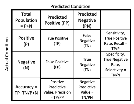
Figure 2: General Confusion Matrix
When this matrix is determined, a large number of different metrics can be calculated. However, there are several most commonly reported and used to evaluate a model, these are Accuracy, Sensitivity, Specificity, Positive Predictive Value & Negative Predictive Value. Depending on the field though, these techniques may be reported differently, or alternatively different metrics may be used. When these main metrics are explained further (below) details will be provided regarding potential alternative names.
Stepping back, let us consider the fundamental confusion matrix and the commonly observed reference labels and shorthands, detailed in the figure below.
- P: Actual Positive
- N: Actual Negative
- PP: Predicted Positive
- PN: Predicted Negative
These core metrics can then be used to calculate the following:
- TP: True Positive
- TN: True Negative
- FN: False Negative (or Type II error)
- FP: False Positive (or Type I error)
This understanding can then be used to calculate the following:
- Sensitivity, True Positive Rate, or Recall: TP / P
- Specificity, True Negative Rate, or Selectivity: TN / N
- Accuracy: TP + TN / P + N
- Positive Predictive Values: TP / PP
- Negative Predictive Values: TN / PN
These values can then be interpreted as such:
- Sensitivity, typical range 0 - 1, score of 1 indicates that all positive cases are correctly identified.
- Specificity, typical range 0 - 1, score of 1 indicates that all negative cases are correctly identified
- Accuracy, typical range 0 - 1, score of 1 indicates that all cases are correctly identified
- Positive Predictive Value, typical range 0 - 1, score of 1 indicates perfect precision, thereby no false positives called
- Negative Predictive Value, typical range 0 - 1, score of 1 indicates no false negatives were found
These metrics individually, or in combination can be used to evaluate a machine learning model.