Advanced Worksheet
Package and Data Loading
As mentioned during the session setup, load the following packages using the library() function. Additionally, as we will be using a data set which contains large numbers, set scipen to 999, within the options() function.
library(tidyverse)
library(caret)
library(tree)
library(rpart)
library(rpart.plot)
library(e1071)

options(scipen = 999)
Furthermore, for the purpose of this session, we will be using data from UC Irvine Machine Learning Repository and in particular the Red Wine Quality Dataset. This can be downloaded from the site directly, or contained in the .zip file.
winequality_red <- read_csv("data/winequality-red.csv")Section 1: Data Preparation for Tree-based Models
Exercise 1: Transform the data: Numeric to Binary
For some tasks you may be required to generate a classification tree, rather than a regression tree. The major difference between these types is that classification trees look to predict a nominal output, whereas regression trees aim to predict a continuous output (numeric). In this case we can actively convert our outcome variable (quality) from a numeric continuous variable (0-8) to a dichotomous variable rating wine as either high (>6) or low (<=6) on this scale.
To do this, (as always) there are multiple options, one of the easiest is the ifelse() function. This function works through providing a binary statement, or threshold, with options being listed if the statement is true or false.
Apply the following code to your data to convert from numeric to binary data. And convert to a factor variable.
winequality_red$quality_bin <- ifelse(winequality_red$quality <= 6,
                                      yes = "low", no = "high")

winequality_red$quality_bin <- factor(winequality_red$quality_bin)
Prior to any models being developed, data must be prepared through splitting in training and testing groups. To do this, two methods can be used, to begin with we will use a manual method in which we split the data by hand.
To ensure we are all using the same data, firstly set the reproducible seed. Personally, I use dates as my seeds, this produces 8 digit seeds which are great for reproducibility.
set.seed(13052006)Most training-test (TT) splits are 80/20, that is 80% training data, 20% testing data.
In our manual method we firstly calculate the number of observations in each set. In this case:
- Training = 1599 x 0.8 = 1279.2
- Testing = 1599 x 0.2 = 319.8
We can adjust these to ensure whole numbers through rounding accordingly.
- Training = 1599 x 0.8 = 1279
- Testing = 1599 x 0.2 = 320
Now we can generate a pair of vectors (train.vec & test.vec) each containing the word “train” or “test” accordingly, to the length provided. These can then be combined as comb.vec of total length 1599, containing both training and testing lists.
train.vec <- rep_len("train", length.out = 1279)
test.vec <- rep_len("test", length.out = 320)

comb.vec <- c(train.vec, test.vec)
Next, using a for loop, as provided below. You can assign each observation as a training or test case, creating a new variable in the process called group.
## Example 1
for(i in 1:1599){
  winequality_red[i,"group"] <- sample(comb.vec, size = 1, replace = FALSE)
}
Note, for more advanced users, this process can be easily completed through skipping the step above and using the following the code in example 2.
## Example 2 (Advanced)
for(i in 1:1599){
  winequality_red[i, "group"] <- sample(c("train", "test"), size = 1, replace = TRUE, prob = c("train" = 0.8, "test" = 0.2))
}
Once these groups are identified they can easily be split using the filter() function. From these divided groups you can then use this data to train and test your Machine Learning Models.
train.dat <- filter(winequality_red, `group` == "train")
test.dat <- filter(winequality_red, `group` == "test")
The alternative, and arguably more direct method uses the createDataPartition() function. In which you skip most of the steps above, simply grouping the data randomly into training or testing data.
## Create Data Partition
train.vec2 <- createDataPartition(
  y = winequality_red$quality, ## Quality is the outcome variable
  p = 0.8, ## p lists the percent to training
  list = FALSE ## Format of the results
)

## Partition The data, based upon the partition
train.dat2 <- winequality_red[train.vec2,]
train.dat2 <- winequality_red[-train.vec2,]
Both methods are acceptable, however the first is useful in understanding the process completed.
Exercise 2: Prepare the data yourself
Using one of the techniques listed above, prepare a training and testing data group. Once split, use summary() to see whether the data is similar. Compare the median, mean and range.
Section 2: My First Decision Tree
Now that the data is prepared, we can begin to examine specific examples. As with most things within R, there are a million different ways to achieve the same goal. In this case, you can use the function rpart() (Package rpart); tree() (Package tree); or train() (Package caret). For this workshop, as the the textbook uses tree(), we will focus on rpart(), providing an alternative. As a general rule, the techniques, and parameter understanding developed here are transferable between different functions.
Exercise 3: Using rpart(), with the formula listed below, generate a classification tree to predict quality.
Formula = quality_bin ~ alcohol + citric acid + pH
Remember to “`” around citric acid, to ensure it recognizes the variable!
Once completed, use rpart.plot() to plot the classification tree.
## Model the Tree
class_tree_1 <- rpart(data = train.dat,
                      formula = quality_bin ~ alcohol + `citric acid` + pH,
                      method = "class")

## Plot the classification tree
rpart.plot(class_tree_1)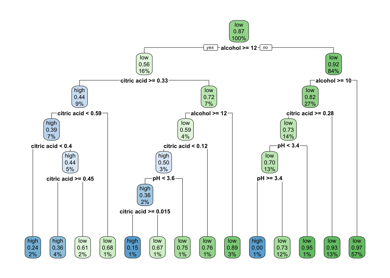
This produces a clear and highly interpretable classification tree, using these variables to classify quality. A similar result can be produced for a regression tree, through adapting the formula swapping quality_bin for quality.
Exercise 4: Using rpart(), generate a regression tree to predict quality.
Remember to use quality rather than quality_bin.
## Model the Tree
reg_tree_1 <- rpart(data = train.dat,
                    formula = quality ~ alcohol + `citric acid` + pH,
                    method = "anova")

## Plot the classification tree
rpart.plot(reg_tree_1)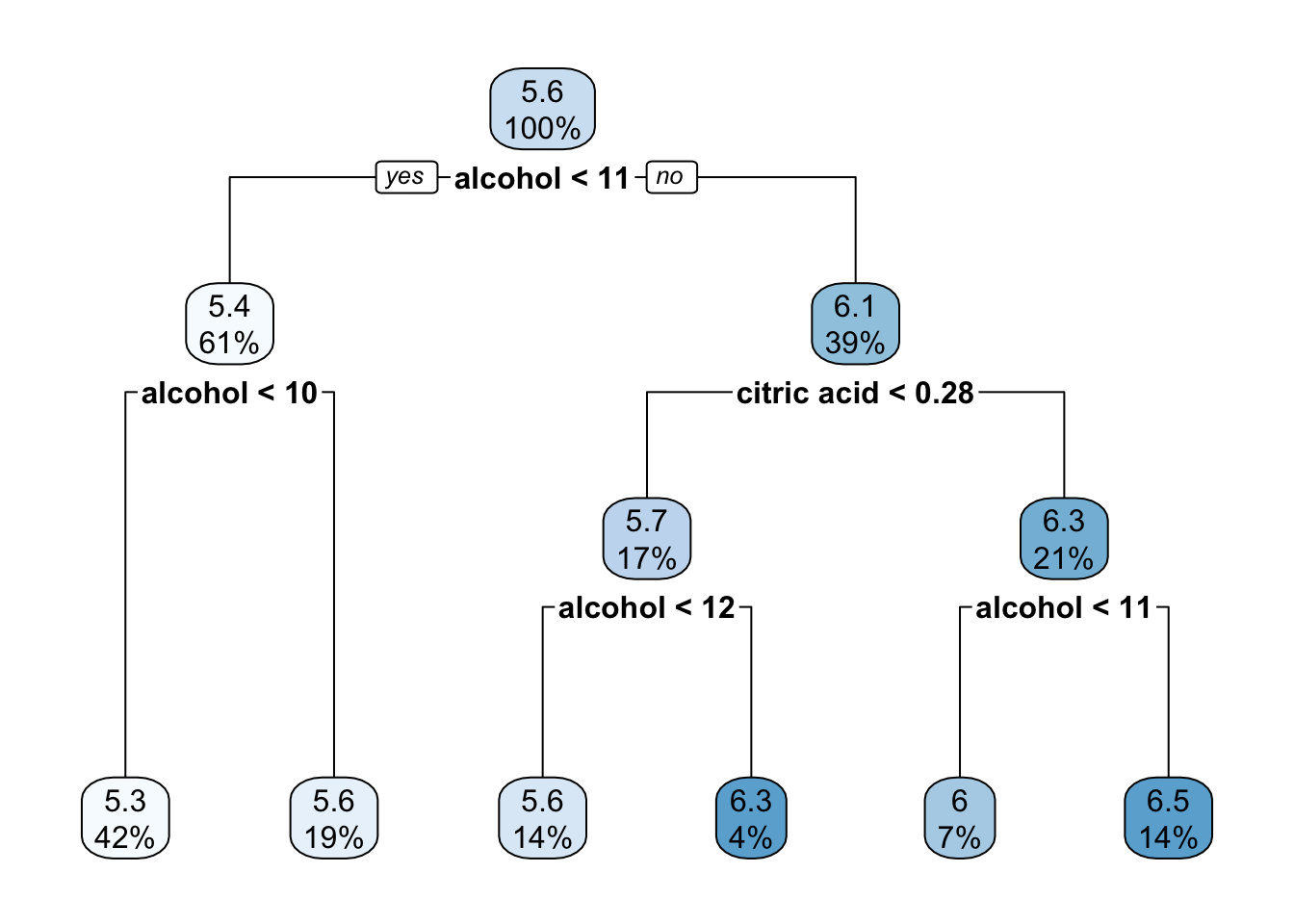
Exercise 5: Compare the plots side by side, which do you think will more accuracy predict red wine quality, the classification or regression tree?
The answer to this is a complex one, and varies based upon the question you would like to answer. We will look into which is more appropriate in the coming sections.
Section 3: Evaluating Tree-based models
In order to evaluate the effectiveness of a devised model, one must first apply the model developed on the training data onto new, novel data, in this case the test data we assigned earlier. From this, we can compare the the predicted outcome to the true outcome using a confusion matrix, to calculate various assessments of evaluation like accuracy.
To apply the model to the training data, we can use the predict() function, which applies the predefined model to new data, in our case being the testing data.
Exercise 6: Using the predict() function, apply both the classification and regression trees to the testing data.
## For classification trees
class_pred <- predict(object = class_tree_1, ## Specify the model here
                      newdata = test.dat, ## Specify the new data here
                      method = "class") ## Specify the type of methodology

## For classification trees
reg_pred <- predict(object = reg_tree_1, ## Specify the model here
                      newdata = test.dat, ## Specify the new data here
                      method = "anova") ## Specify the type of methodology
When we use the predict function, this applies the new data provided to the specified object model, in order to predict the outcome. From this depending on what type of model we have used, we can evaluate its performance.
Before any evaluations can take place, some cleaning and manipulation must be completed. Firstly, for classification prediction a probability is produced for each available option, as such we must specify which is the predicted category each observation falls into. This can be done using another for loop and associated if statements as below:
## Convert the predicted information to a dataframe
class_pred <- as.data.frame(class_pred)

## For each row in in the predicted class, if the probability is greater for high than low, then list high as the predicted.
for(i in 1:nrow(class_pred)){
  if(class_pred[i,1] > class_pred[i,2]){
    class_pred[i,"pred"] <- "high"
  } else {
    class_pred[i,"pred"] <- "low"
  }
}

## Convert to a factor
class_pred$pred <- factor(class_pred$pred)
Once this manipulation is completed, you can use the function confusionMatrix() which compared the predicted against the actual observations in order to evaluate the model.
Exercise 7: After manipulating the predicted class data as above, use the function confusionMatrix() to evaluate this model
confusionMatrix(data = class_pred$pred, ## Specify the predicted data and specifically the output
                reference = test.dat$quality_bin) ## Specify the reference data and specifically the output
## Confusion Matrix and Statistics
##
## Reference
## Prediction high low
## high 7 14
## low 39 244
##
## Accuracy : 0.8257
## 95% CI : (0.7782, 0.8666)
## No Information Rate : 0.8487
## P-Value [Acc > NIR] : 0.8836254
##
## Kappa : 0.1261
##
## Mcnemar's Test P-Value : 0.0009784
##
## Sensitivity : 0.15217
## Specificity : 0.94574
## Pos Pred Value : 0.33333
## Neg Pred Value : 0.86219
## Prevalence : 0.15132
## Detection Rate : 0.02303
## Detection Prevalence : 0.06908
## Balanced Accuracy : 0.54896
##
## 'Positive' Class : high
## When running this function, it produces a large amount of different statistical information, these are broken down further in Learning Material: Evaluating Models.
In comparison, to evaluate the fit of regression trees, we use Root Mean Squared Error or RMSE. Which is a single measure of the absolute deviation from the predicted line the observed area. With the smaller this value being, the better fit this model is.
To calculate the RMSE, the function RMSE() can be used, similar to the confusionMatrix function, this also uses data and reference as its inputs.
Exercise 8: Using the function RMSE() evaluate the Regression Tree Model
RMSE(pred = reg_pred, # Predicted
     obs = test.dat$quality) # Observed
## [1] 0.7712802Section 4: Review & Comparison
Exercise 9: Using all the knowledge from today’s session, and that available from the Learning Materials tab, run additional regression and classification trees, using as much or as little of the data set provided as you wish, and compare which combination of variables is best at predicting quality.
For your learning, I would suggest repeating Section 1, or if time is limited using the training and test data previously generated.
Please note, during the next installment of this series: Introduction to Machine Learning: Tree-based Models 2, we will be exploring alternative ways to increase prediction accuracy including pruning.